Election prediction using Elo

Overview

This post is a re-adaptation and R-implementation of my previous post on a fun modeling project using Elo to predict the latest 2020 presidential elections. The previous implementation was done in Julia and can be found in this interactive Pluto.jl document. You can find the source code for the Julia implementation here. For this exercise, first let’s load our libraries:

Code

library(tidyverse)
library(lubridate)
library(jsonlite)
library(glue)
library(ggthemes)
library(showtext)
font_add_google("Roboto Slab")
showtext_auto()

What is an Elo model?

The elo rating system is a method developed by Arpad Elo in order to rank players by ability in a zero sum game. Elo has been used in various contexts, most famously the way to rank chess players through the UCSF and FIDE systems. Elo has been used in modern contexts as well, from Tinder to World of Warcraft. A really nice attribute about Elo is that a difference in rankings can be translated to a probability. Let’s assume a focal player \(A\) with rank \(R_A\) is facing up against opponent \(B\) with rank \(R_B\). The expected “score” \(E_A\) of player \(A\) in the match can be defined as:

\[E_A = \frac{1}{1 + 10^{(R_B - R_A)/400}} = \frac{1}{1 + 10^{-(R_A - R_B)/400}}\]

Recall that the standard logistic function is \(\frac{1}{1 + e^{-x}}\). You can see that there are tons of similarities between the standard logistic function and the function for the expectation of player \(A\)’s score, with the exception being the exponential constant \(e\). This is because while elo probabilities are log-odds, they are not natural log based but rather based on base 10. There are easy conversions between the base 10 and base \(e\), which allows sports statisticians to perform logistic regression on elo rankings. However, that is a bit beyond the focus of this project.

The elo model updates the ranking of the person after each match. For our focal player \(A\), the rankings are updated as:

\[R_A* = R_A + K \cdot (outcome - E_A)\] where \(K\) is the \(K\)-factor controlling the relative gains and losses of elo points. The variable outcome here is a binary variable (1 if player \(A\) wins). Think of this similar to how you would use a binary cross-entropy loss to train a model that outputs an odds (such as a logistic regression) instead of true binary values. In this case, ranking updates are based on the difference between the true outcome and the expected outcome \(E_A\). Let’s define a couple of functions reflecting the ideas above:

Code

# Calculate win probabilities from two rankings  
win_prob <- function(r1, r2){
  x1 <- 10^((r2 - r1)/400)
  p1 <- 1/(1 + x1)
  p2 <- 1 - p1
  return(list(p1 = p1 , p2 = p2))
}

# Back transform from probability to difference in rankings 
back_transformation <- function(prob){
  diff <- 400 * log((1/prob) - 1,base = 10)
  # we want difference between the focal person, which means we have to invert this
  return(diff * -1)
}

The first function, win_prob calculates the win probability given two rankings. It outputs a list with p1 being the win probability of the focal player 1. The second function, back_transformation, takes in the probability and returns a difference in rankings.

To test and see whether our model is correct, let’s compare to a reference. According to this website, a win probability of 0.76 for focal player 1 would be a result of 200 elo difference. Let’s try it out!

Code

glue("Win probability of 76% converts to an elo difference of {diff}", diff = back_transformation(0.76))

Win probability of 76% converts to an elo difference of 200.240940227674

So our elo formulation so far is correct.

The US presidential election as a pseudo-sports contest

The US presidential election is a surprisingly appropriate context to use elo. In this election, two candidates compete for the “title” of the President of the United States. Polling data is collected regularly, which can act as “matches” where the two candidates can test their “mettle” before the final election day. Furthermore, the structure of the election, a winner-take-all Electoral College system, makes it even closer to being a sports match.

In this instance, elo system is applied to model the probability of winning an election. Weekly average polling results are used as proxy for “games”. After each weekly poll, the candidate gains or lose elo based on whether they win or lose (polling average > 50%) and how much did they win (or lose) by. Some major caveats and assumptions:

• First, this model is for fun, and does not consider variables such as demographics, economics, recent news, etc., which are considered part of the fundamentals portion of any reliable forecasting model. Since the model ingests polling averages from FiveThirtyEight, it does account for quality of polling and other associated factors as a proxy.

• Second, the model does not account for random effects occuring at the state level or across time, as each unit of polling is considered to be independent.

• Third, the model rewards consistent polling, and rewards them with higher probability of winning. I would say this is a reasonable assumption as performance in the polls with high margins often indicate a victory in that jurisdcition. However, as many consumers of election modelling know, factors such as close to election day scandals or turnout would affect the final results and violate this assumption.

Methods

“Training” data

Let’s start our modeling exercise by reading in basic polling data from FiveThirtyEight. Here, we simplify things a little bit. First, we do not consider the split votes of the states of Nebraska and Maine, and second, we only focus on the adjusted percentage scores, which usually accounts for polling reliability.

Code

data <- read.csv(file = "data/presidential_poll_averages_2020.csv")
proc_data <- data %>% as_tibble() %>% mutate(modeldate = as_date(strptime(modeldate, format = "%m/%d/%Y"))) %>% # reformat names
  mutate(candidate_name = case_when(
    candidate_name == "Convention Bounce for Joseph R. Biden Jr." ~ "Joseph R. Biden Jr.",
    candidate_name == "Convention Bounce for Donald Trump" ~ "Donald Trump", 
    TRUE ~ candidate_name
  )) %>% mutate(week = week(modeldate)) %>% filter(!state %in% c("NE-1", "NE-2", "ME-1", "ME-2", "National")) %>% # for simplicity
  group_by(state, week, candidate_name) %>% # get week 
  summarise(poll_avg = mean(pct_trend_adjusted)) # average per week 
rmarkdown::paged_table(proc_data)

Prior information for initial elo seeding

Just having an elo model is not enough! We want to seed our “players” with some elo first. The easiest way is to seed both candidates with an elo of 1000, but that doesn’t account for each candidate’s advantage at each state due to their political affiliation. Here, we decided to take a simple solution and take the election results from the 2016 election. Based on the margin of victory, we will use the back_transformation function to calculate a difference in elo and use that as a seed. For example, if Donald Trump won state X with 76% of the votes, then he would start with 1200 elo compared to Joe Biden’s 1000 elo. As such, we are able to incorporate some prior information. We want polling to be good enough to overcome this inherent advantage.

Code

# Function to convert abbreviation to state name
get_stname <- function(state_abb){
  if (state_abb == "DC"){
    name <- "District of Columbia"
  } else {
    name <- state.name[grep(state_abb, state.abb)]
  }
  if (rlang::is_empty(name)){
    return(NA_character_)
  } else {
    return(name)
  }
}
# Prior information 
prior <- read.csv(file = "data/returns-2016.csv") %>% as_tibble()

# convert state abbreviation to name, renormalize to two party candidates, then back transform prob to difference in elo
prior <- prior %>% mutate(state = map_chr(state_abbreviation, ~get_stname(.x))) %>% 
  mutate(Clinton = Clinton/(Clinton + Trump), Trump = Trump/(Clinton + Trump)) %>% 
  select(-c(state_abbreviation, Other)) %>% 
  mutate(elo_diff = back_transformation(Clinton))
rmarkdown::paged_table(prior)

Incorporating margin of victory

A lot of elo models also incorporate something called the margin of victory. Margin of victory (mov) scales elo gains and losses based on how well the player performed. A knock-out match from an underdog would result in a massive gain in elo, compared to if that match was a close one. We try to incorporate margin of victory into our elo update calculation by modifying the K-factor with a linear adjustment \[K_{eff} = K * mov\] where \[mov\] is the margin of victory. This means that the “winning” candidate will gain points as a proportion of K that is equal to their margin of polling victory. As such, we increase values of K significantly to compensate for the low gains in elo when margins can be 1 percent. This also prevents polling results from driving elo scores to crazy levels.

Taking that into account, here’s out update function.

Code

# Update elo using those rankings  

update_elo <- function(r1, r2, outcome, mov, K=30){
  probs <- win_prob(r1, r2)
  p1 <- probs$p1
  p2 <- probs$p2
  K = K * mov # K-gains as a proportion of margin of victory  
  r1_new <- round(r1 + K*(outcome - p1), digits = 0)
  r2_new <- round(r2 + K*((1 - outcome) - p2), digits = 0)
  return(list(r1 = r1_new, r2 = r2_new))
}

Getting elo sequence

The general gist of the model would be getting the elo sequence for each state based on weekly average polling, with prior information from the 2016 election. We’re going to choose the Democratic candidate as the focal candidate, with rankings equals r1. With that in mind, a wrapper function that performs this for each state.

Code

get_sequence <- function(proc_data, prior, st, init=1000, K = 50){
  df <- proc_data %>% filter(state == st) # filter by state
  weeks <- unique(df$week) # get all unique weeks 
  elo <- vector(mode = "list", length = length(weeks) + 1) # initialize elo vector
  prior_diff <- prior %>% filter(state == st) %>% pull(elo_diff)
  # if Trump won state then prior_diff < 0 since Democrats are the focal candidate
  if (prior_diff < 0){
    elo[[1]] <- tibble(
      DT_elo = init + abs(prior_diff),
      JB_elo = init
    )
  } else if (prior_diff > 0){
    elo[[1]] <- tibble(
      DT_elo = init,
      JB_elo = init + abs(prior_diff)
    )
  } else {
    elo[[1]] <-  tibble(
      DT_elo = init,
      JB_elo = init
    )
  }
  # iterate 
  for (i in 2:length(elo)){
    elos <- update_elo(r1 = elo[[i-1]]$JB_elo, 
                       r2 = elo[[i-1]]$DT_elo,
                       outcome = df$win[i-1], 
                       mov = df$mov[i-1], K = K)
    elo[[i]] <- tibble(
      DT_elo = elos$r2,
      JB_elo = elos$r1,
    )
  }
  seq <- do.call(rbind, elo)
  weeks <- c(min(weeks)-1, weeks)
  seq <- seq %>% mutate(state = rep(st, length(elo)), week = weeks)
  seq <- seq %>% select(state, week, DT_elo, JB_elo) %>% 
    pivot_longer(c(DT_elo, JB_elo), names_to = "candidate", values_to = "elo") %>% 
    mutate(candidate = recode(candidate, DT_elo = "DT", JB_elo = "JB")) %>% 
    pivot_wider(names_from = candidate, values_from = elo)
  return(seq)
}

The implementation for this is a bit weird, since we have a time 0 where the candidates are seeded. But before we apply this to our data, first let’s process further the basic polling and assigning a win or loss based upon the polling percentages to generate our \(outcome\). If the poll is tied, a random draw from the binomial distribution is performed.

Code

proc_data <- proc_data %>% 
  mutate(candidate_name = case_when(candidate_name == "Donald Trump" ~ "DT", TRUE ~ "JB")) %>% 
  pivot_wider(names_from = "candidate_name", values_from = "poll_avg") %>% 
  mutate(win = case_when(JB > DT ~ as.integer(1), 
                         JB < DT ~ as.integer(0), 
                         JB == DT ~ rbinom(1,1,0.5))) %>% 
  mutate(mov = abs(DT - JB)/100)
rmarkdown::paged_table(proc_data)

Applying our elo sequences model for all states.

Code

get_elo_all_states <- function(proc_data, prior, K=50, init=1000){
  states <- unique(proc_data$state)
  data <- vector(mode = "list", length = length(states))
  for (i in seq_len(length(states))){
    data[[i]] <- get_sequence(proc_data, prior, states[i], K = K, init = init)
  }
  return(do.call(dplyr::bind_rows, data))
}

elo_sequences <- get_elo_all_states(proc_data, prior)
elo_sequences <- elo_sequences %>% rowwise() %>% mutate(prob = win_prob(r1 = JB, r2 = DT)$p1)
rmarkdown::paged_table(elo_sequences)

Final probabilities using Monte Carlo simulations

To determine the final probability of winning the election, we take our state-level probabilities and simulate binomial draws with our probabilities. This is similar to how FiveThirtyEight performs their final modelling as well. The final win chance is therefore the the number of simulations where a focal candidate (in this case Biden) gains 270 or more Electoral Votes.

Processing electoral votes data

Code

electoral_votes <- jsonlite::fromJSON("data/electoral_votes.json")
electoral_votes <- do.call(rbind, electoral_votes) 
electoral_votes <- electoral_votes %>% as.data.frame() %>% rename("votes" = "V1") %>% 
  rownames_to_column(var = "state") %>% 
  mutate(state = map_chr(state, get_stname)) %>%
  na.omit() %>% as_tibble()

Let’s create another wrapper function that wraps all of this together in one go:

Code

elo_predict <- function(proc_data, prior, e_votes, K = 50, init = 1000, n_iter = 1000){
  # first, let's get all elo sequences 
  elo_sequences <- get_elo_all_states(proc_dat = proc_data, prior = prior, K = K, init = init)
  # then, let's get probabilities from them 
  elo_sequences <- get_elo_all_states(proc_data, prior)
  elo_sequences <- elo_sequences %>% rowwise() %>% mutate(prob = win_prob(r1 = JB, r2 = DT)$p1)
  # then, let's retrieve the probabilities by state at the last week 
  # (which.max allows for selecting the most recent week)
  suppressMessages(probs <- elo_sequences %>% group_by(state) %>% summarise(prob = prob[which.max(week)]))
  # merge electoral votes with probability data 
  probs <- left_join(probs, e_votes, by = "state")
  # predict and multiply with votes 
  suppressMessages(preds <- map_dfc(seq_len(n_iter), ~{
    map_int(probs$prob, ~rbinom(1,1,.x)) * probs$votes
  }))
  # rename 
  names(preds) <- paste0("sim_",seq_len(n_iter))
  # retrieve state names and swtich columns
  preds <- preds %>% mutate(state = probs$state) %>% select(state, everything())
  return(list(preds = preds, elo_seq = elo_sequences))
}

Results

Now that we have everything set up, let’s perform some predictions!
We use the default \(K\)-factor of 50 and the initial elo seeding of 1000 with 1000 simulations. Since elo operates mostly from the differences in elo rankings, the initial elo seeding is not as important.

Code

pred <- elo_predict(proc_data = proc_data, prior = prior, e_votes = electoral_votes, K = 50, init = 1000)
rmarkdown::paged_table(pred$preds)

With our predictions, we can tally up the number of times the focal candidate JB wins over 270 electoral votes, which can get us an estimate of the overall probability. We can also do some bootstrap resamplings of the already generated 1000 simulations to get an bootstrapped interval.

Code

vote_counts <- colSums(pred$preds[,-1]) %>% unname()
probability <- round((length(which(vote_counts >= 270))/1000)*100, digits = 2)

boot <- map_dbl(seq_len(1e4), ~{
  counts <- sample(vote_counts, size = 1000, replace = T) 
  round((sum(counts >= 270)/1000)*100, digits = 2)
})

glue("Win probability of Biden is {prob}% ({lower}% - {upper}%)", 
     prob = probability, lower = quantile(boot, 0.025), upper = quantile(boot, 0.975))

Win probability of Biden is 80% (77.5% - 82.4%)

This is a pretty reasonable assumption. Let’s explore the uncertainty around our probability model a bit further. Let’s first visualize the distribution of votes across all simulations

Code

qtile <- quantile(vote_counts, probs = c(0.025, 0.975))

plt <- qplot(x = vote_counts, geom = "histogram", fill = I("#5657B8"), alpha = I(0.8), binwidth = 10) + 
  theme_bw() + 
  labs(x = "Electoral Vote Counts", y = "Frequency", title = "Distribution of total electoral vote counts",
       subtitle = "1000 simulations") + 
  geom_vline(xintercept = qtile[1], col = "red", size = 1.5) + 
  geom_vline(xintercept = qtile[2], col = "red", size = 1.5) + 
  annotate(geom = "curve", x = 175, y = 75, xend = qtile[1], yend = 50, 
           curvature = 0.3, arrow = arrow(length = unit(2, "mm"))) +
  annotate(geom = "text", x = 175, y = 83, label = glue("0.025 quantile \n {val}", val = qtile[1])) +
  annotate(geom = "curve", x = 420, y = 75, xend = qtile[2], yend = 50, 
           curvature = 0.2, arrow = arrow(length = unit(2, "mm"))) +
  annotate(geom = "text", x = 420, y = 83, label = glue("0.075 quantile \n {val}", val = qtile[2])) +
  theme(text = element_text(famil = "Roboto Slab", size = 13))
print(plt)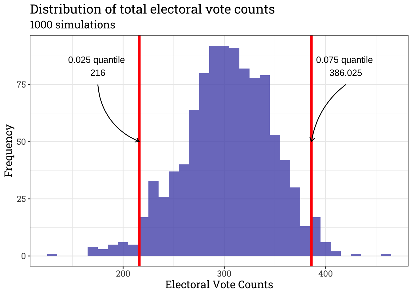

We can visualize the trajectory of elo for each state. Let’s take three states: California, Pennsylvania and Arkansas. These three states represents three types of states you would usually see: solidly blue, swing, and solidly red.

Code

seq <- pred$elo_seq
seq <- seq %>% filter(state %in% c("California", "Pennsylvania", "Montana"))
seq <- seq %>% pivot_longer(c(DT, JB))
ggplot(seq, aes(x = week, y = value, col = name)) + geom_line() + geom_point() + 
  facet_grid(state~., scales = "fixed") + 
  scale_color_brewer(palette = "Set1", labels = c("Donald Trump", "Joe Biden")) + theme_bw() + 
  labs(y = "Elo sequence", x = "Polling week", col = "Candidate", 
       title = "Weekly elo rankings for each candidate") + theme(text = element_text(family = "Roboto Slab"))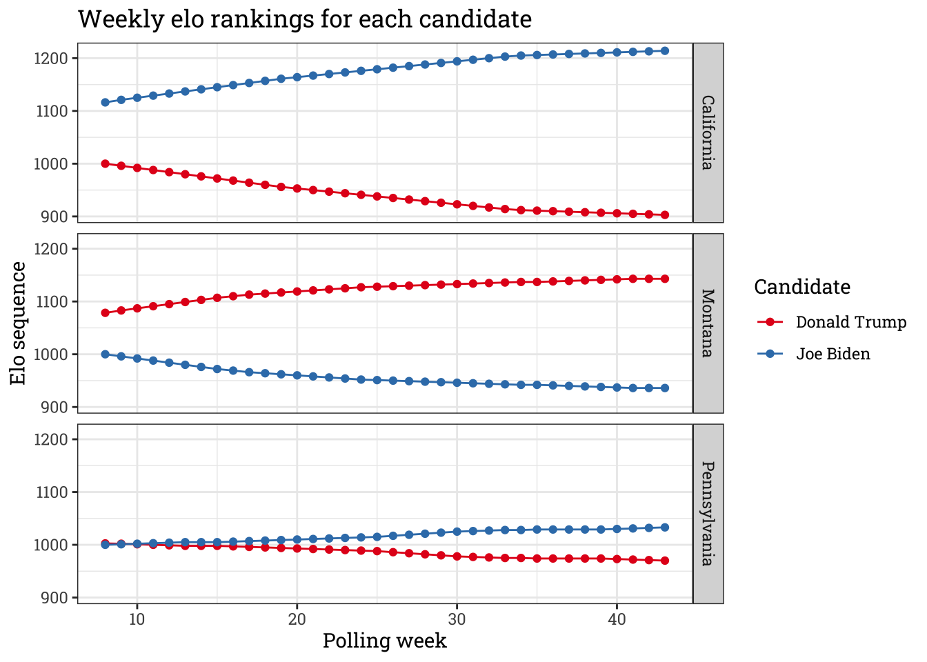

The elo rankings here makes sense. For states like California and Montana whose political affiliation is well known, the elo difference is larger, and continue to increase throughout the week due to good polling. The margin of victory also scales accordingly, where the rate of elo gain for Biden in California and Montana are really high. Conversely, Pennsylvania, while right now heading in Biden’s direction, do not change as much. The margin of victory was probably too small to generate a wide gap as that of the other two states, indicating a close race. However, it seems that the polling is good enough for Joe Biden to overcome the results of the 2016 election.

Finally, let’s generate a fun visual similar to FiveThirtyEight’s bubble plots!

Code

set.seed(1234)
counts <- tibble(counts = sample(vote_counts, size = 100, replace = T)) %>% arrange(desc = TRUE) %>% 
  mutate(cat = rep("simulation", 100)) %>% mutate(counts = counts - (538 - counts)) %>% 
  mutate(win = case_when(
    counts > 0 ~ "Win",
    counts == 0 ~ "Tie",
    counts < 0 ~ "Loss"
  ))
ggplot(counts, aes(x = cat, y = counts, col = win)) + geom_jitter(size = 5, alpha = 0.8) + theme_minimal() + 
  coord_flip() + geom_hline(yintercept = 0) + 
  theme(axis.line.y = element_blank(), axis.title.y = element_blank(), axis.ticks.y = element_blank(), 
        axis.text.y = element_blank(), panel.grid.major = element_blank(), 
        text = element_text(family = "Roboto Slab"),
        panel.grid.minor = element_blank()) +
  scale_y_continuous(breaks=c(-300,-150,0,150,300)) + scale_color_brewer(palette = "Set1") +
  labs(y = "Electoral vote differences", col = "Result for Biden") +
  annotate("text", y = 150, x = 1.5, 
           label = glue("Chance of winning \n {val} in 100", val = sum(counts$counts >= 0)))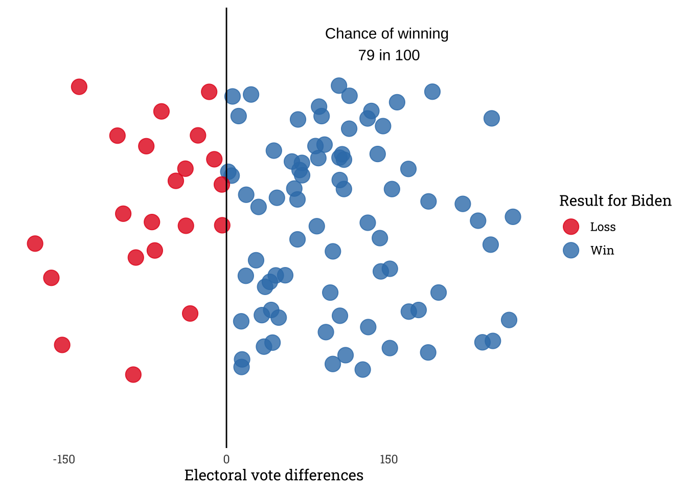 

Conclusions

While this model is something I made for fun, it’s cool to learn about elo as a way to explore topics relating to modelling competitions such as sports. The elo sequence somehow strangely makes sense in this case, presenting a pretty acceptable picture of the electoral landscape. Some additional things that could be explored further:

• A random effects logistic regression model for elo can be fitted to not just control for temporal effects (since our data is longitudinal), but can also allow the mean of elo scores per week to vary with other predictors that are considered core in the election forecasting field.
  
• A better way to incorporate margin of victory can help with states just converging to almost 100% win probability.
  
• More sensitivity analysis with K-factors and adjusting elo gains and losses.

That said, this was super fun! Hope this write-up was enjoyable!

Citation

BibTeX citation:

@online{nguyen2021,
  author = {Quang Nguyen},
  title = {Election Prediction Using {Elo}},
  date = {2021-01-10},
  langid = {en}
}

For attribution, please cite this work as:

Quang Nguyen. 2021. “Election Prediction Using Elo.” January 10, 2021.